Superfluid density

The normal and superfluid fractions of a liquid can be obtained by measuring the momenta of inertia of a rotating bucket. Consider a liquid which is inserted between two cylindrical walls of radii $R$ and $R+d$. If $d \ll R$ then the system can be described as moving between two planes. Let us denote by $E_{{\upsilon}}$ the ground state energy of the system in equilibrium with the walls which move with velocity ${\upsilon}$ and $E_0$ the ground state energy of the system at rest. The difference between the energies $E_{{\upsilon}}$ and $E_0$ is due to the superfluid component, which remains immobile in contrast to the normal component which is carried along by the moving walls. Thus, the superfluid fraction $\rho _s/\rho$ can be defined as

$$\frac{N m {\upsilon}^2}{2} \frac{\rho_s}{\rho} = E_{{\upsilon}} - E_0$$ (3.48)

Let us introduce the wave-functions $f_0$ and $f_{{\upsilon}}$ related to the wave-functions of the system in the reference frames at rest and in motion.

$$f_0({\bf R}, t) = \psi_T({\bf R}) \phi_0({\bf R}, t),$$ (3.49)

$$f_{{\upsilon}}({\bf R}, t) = \psi_T({\bf R}) \phi_{{\upsilon}}({\bf R}, t)$$ (3.50)

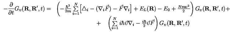
These wavefunctions satisfy the Schrödinger equation with the following Hamiltonians

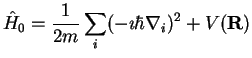
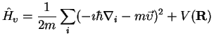
$$\hat H_0 = \frac{1}{2m} \sum\limits_i (-\imath \hbar \nabla_i)^2 + V({\bf R})$$ (3.51)

for the reference frame at rest and

$$\hat H_{{\upsilon}} = \frac{1}{2m} \sum\limits_i (-\imath \hbar \nabla_i -m \vec{{\upsilon}} )^2 + V({\bf R})$$ (3.52)

for the reference frame at moving with velocity ${\upsilon}$. In the reference frame at rest one has

$$-\frac{\partial}{\partial t} f_0({\bf R}, t) = -\frac{\hbar^2}{2m... ...\Bigl(\vec F f_0({\bf R},t)\Bigr)\biggr] + (E_L({\bf R}) - E_0) f_0({\bf R}, t)$$ (3.53)

The Schrödinger equation in the moving frame is instead

$$\begin{array}{ll} \displaystyle-\frac{\partial}{\partial t} f_{{\... ...athstrut {\upsilon}} \vec{\mathstrut F} f_{{\upsilon}} ({\bf R}, t) \end{array}$$ (3.54)

Looking at (3.53) and (3.54) it is easy to write the Bloch equations for the Green's functions in the rest frame $G_0({\bf R}, {\bf R'}, t)$ and in the moving frame $G_{{\upsilon}}({\bf R}, {\bf R'}, t)$

$$-\frac{\partial}{\partial t} G_0({\bf R}, {\bf R'}, t) = \left(-\... ...F) - \vec F\nabla_i\Bigr] + E_L({\bf R}) - E_0\right) G_0({\bf R}, {\bf R'}, t)$$ (3.55)

and

$$\begin{array}{lc} \displaystyle-\frac{\partial}{\partial t} G_{{\... ...\vec{{\upsilon}} \vec F\right) G_{{\upsilon}}({\bf R}, {\bf R'}, t) \end{array}$$ (3.56)

In general the wavefunction $\psi({\bf R},t)$ of the system satisfies the Schrödinger equation (3.2) and its evolution in time is described by

$$\psi ({\bf R},t) = e^{-(\hat H - E)t} \psi ({\bf R},0)$$ (3.57)

The wavefunctions $f$ evolves in time as

$$f({\bf R},t) = e^{-At} f({\bf R},0)$$ (3.58)

so, substitution of (3.49) or (3.50) into (3.58) gives

$$\psi_T({\bf R})\psi({\bf R},t) = e^{-At}\psi_T({\bf R})\psi({\bf R},0)$$ (3.59)

Combining together (3.57) and () one has

$$e^{-At} = \psi_T({\bf R}) e^{-(\hat H - E)t} \psi_T^{-1}({\bf R}) = B e^{-(\hat H - E)t} B^{-1},$$ (3.60)

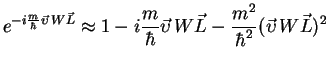
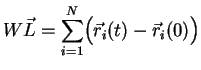
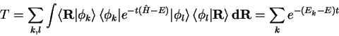
where the operator $B$ is defined as $B\vert\psi\rangle = \sum_{\bf R} \psi({\bf R})\, \langle {\bf R}\vert\psi\rangle~\vert{\bf R}\rangle$. Let us calculate the trace of the Green's function. From (3.60) it follows that the trace $T$ of the Green's function is equal to

$$T = \int\!G_0({\bf R}, {\bf R}, t)\,{\bf dR} = \int\langle... ...rt B e^{-t(\hat H - E) B^{-1}}\vert {\bf R} \rangle\,{\bf dR}$$ (3.61)

Here it is possible to use the permutation property of the trace $\mathop{\rm tr}\nolimits (AB) = \mathop{\rm tr}\nolimits (BA)$

$$T = \int \langle {\bf R}\vert e^{-t(\hat H - E)}\vert {\bf R} \rangle\,{\bf dR}$$ (3.62)

This formula means that the trace of the Green's function is unaffected by the presence of the trial wavefunction $\psi_T$.

$$T = \sum\limits_{k,l} \int \langle{\bf R}\vert\phi_k\rangl... ...l\vert{\bf R}\rangle\,{\bf dR} = \sum\limits_k e^{-(E_k-E)t}$$ (3.63)

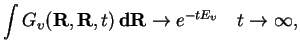
After long enough time of evolution the traces of the Green's function $G_0$ is fixed by the ground state energy

$$\int G_0({\bf R}, {\bf R}, t)\,{\bf dR}\to e^{-E_0t}, \quad t\to\infty,$$ (3.64)

Approximation (3.64) is valid for times $t$ such that

$$t \gg 1 / E_0$$ (3.65)

Analogously, the trace of $G_{{\upsilon}} ({\bf R, R},t)$ is fixed by the ground state energy $E_{{\upsilon}}$ in the moving frame

$$\int G_{{\upsilon}}({\bf R, R},t)\,{\bf dR}\to e^{-t E_{{\upsilon}}}\quad t\to\infty,$$ (3.66)

The Green's function has to comply with periodic boundary conditions, i.e. it must remain the same if one of the arguments is shifted by the period $\vec L$

$$G_0(\vec r_1, ..., \vec r_i + \vec L, ..., \vec r_N,~{\bf R'},~t) = G_0(\vec r_1, ..., \vec r_i, ..., \vec r_N,~{\bf R'},~t),$$ (3.67)

$$G_{{\upsilon}}(\vec r_1, ..., \vec r_i + \vec L, ..., \vec r_N,~{\bf R'},~t) = G_{{\upsilon}}(\vec r_1, ..., \vec r_i, ..., \vec r_N,~{\bf R'},~t)$$ (3.68)

Let us define a new Green's function $\tilde G({\bf R}, {\bf R'}, t)$ in such a way that

$$G_{{\upsilon}}({\bf R, R'},t) = exp\left(i\frac{m}{\hbar} \vec{{\... ...} \sum\limits_i (\vec r_i - \vec r_i\mathstrut')\right) \tilde G({\bf R, R'},t)$$ (3.69)

The Green's function $\tilde G({\bf R, R'}, t)$ satisfies the same Bloch equation (3.55) as $G_0({\bf R}, {\bf R'}, t)$, but the boundary conditions differ from (3.67, 3.68) by the presence of a phase factor

$$\tilde G(\vec r_1, ..., {\vec r_i+\vec L}, ..., \vec r_N,~{\bf R'... ...hstrut L}\right) \tilde G(\vec r_1, ..., \vec r_i, ..., \vec r_N,~{\bf R'},~t),$$ (3.70)

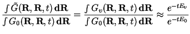
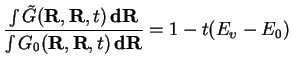
Results (3.64) and (3.66) give the following relation

$$\frac{\int \tilde G({\bf R, R},t)\,{\bf dR}}{\int G_0({\bf R, R},... ... G_0({\bf R, R},t)\,{\bf dR}} \approx \frac{ e^{-t E_{{\upsilon}}}}{e^{-t E_0}}$$ (3.71)

By assuming that $t (E_{{\upsilon}} - E_0) \ll 1$ one gets

$$\frac{ e^{-t E_{{\upsilon}}}}{e^{-t E_0}} \approx 1 - t(E_{{\upsilon}} - E_0)$$ (3.72)

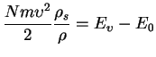
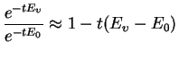
The ratio of the traces is related to the energy difference

$$\frac{\int\tilde G({\bf R, R},t)\,{\bf dR}}{\int G_0({\bf R, R},t)\,{\bf dR}} = 1 - t(E_{\upsilon}- E_0)$$ (3.73)

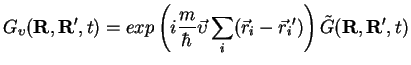
The Green's function $\tilde G$ coincides with $G_0$ apart when the boundary conditions are invoked. Let us introduce the winding number $W$ [25], which counts how many times the boundary conditions were used during the time evaluation

$$1 - t(E_{\upsilon}- E_0) = \frac{\int \vert f({\bf R},t)\vert^2 e... ...vec{{\upsilon}}\,W\vec L}\,{\bf dR}} {\int \vert f({\bf R},t)\vert^2\,{\bf dR}}$$ (3.74)

In the case of slowly moving walls, i.e. when $\vec{{\upsilon}}\,\frac{m}{\hbar} W\vec L \ll 1$, the exponential can be expanded in a Taylor series

$$e^{-i \frac{m}{\hbar}\vec{{\upsilon}}\,W\vec L} \approx 1 -i\frac... ...r}\vec{{\upsilon}}\,W\vec L - \frac{m^2}{\hbar^2} (\vec{{\upsilon}}\,W\vec L)^2$$ (3.75)

Let us define $W$ through the distance the particles have gone during the time $t$

$$W\vec L = \sum\limits_{i = 1}^N\Bigl(\vec r_i(t) - \vec r_i(0)\Bigr)$$ (3.76)

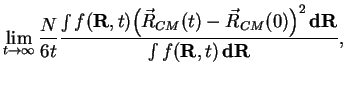
The average value of the linear term is equal to zero and the final result is

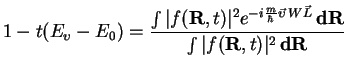
$$\frac{\rho_s}{\rho} = \frac{2m}{\hbar^2} \frac{1}{6 N} \lim\limit... ...({\bf R},t)\vert^2 (WL)^2\,{\bf dR}} {\int \vert f({\bf R},t)\vert^2\,{\bf dR}}$$ (3.77)

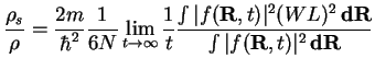
An interpretation of this result is that the superfluid fraction is equal to the ratio between the diffusion constant $D_{{\upsilon}}$ of the center of the mass of the system and the free diffusion constant $D_0$^3.1

$$\frac{\rho_s}{\rho} = \frac{D_{{\upsilon}}}{D_0},$$ (3.78)

where the diffusion constants are defined as

$$D_0 = \frac{\hbar^2}{2m} ,$$ (3.79)

$$D_{{\upsilon}} = \lim\limits_{t \to \infty} \frac{N}{6t} \frac{\int f({\bf R}, t)\... ...vec R_{CM}(t)-\vec R_{CM}(0)\Bigr)^2 \,{\bf dR}} {\int f({\bf R},t)\,{\bf dR}},$$ (3.80)

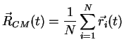
where the center of the mass of the system is

$$\vec R_{CM}(t) = \frac{1}{N} \sum\limits_{i=1}^N \vec r_i(t)$$ (3.81)

By calculating the ratio $D_{\upsilon}/D_0$ as a function of time one finds that this ratio starts from $1$ at small time step, decreases and finally reaches a constant plateau, In practice the best way of finding the asymptotic value is to fit the ration $D_{\upsilon}/D_0$ with the function $C_0+C_1(1-exp(-C_2t))/t$, where $C_0$, $C_1$, $C_2$ are fitting parameters [26]. It is worth to remind that the calculation of $\rho _s/\rho$ is independent of the choice of the trial wave-function and similarly to the calculation of energy the superfluid fraction is a pure estimator.