
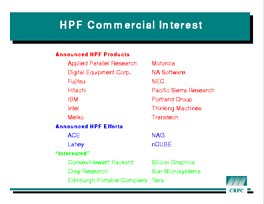
 High Performance Fortran (HPF) was defined in 1993 to provide a portable language
for programming scientific applications on parallel computers. Since
then, many companies have begun to offer HPF compilers, converters,
training, and other products. This tutorial presents many features of
HPF. But first, we give a short introduction to parallel machines and
their languages.
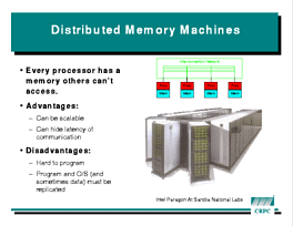 There are several classes of parallel machines, including distributed
memory machines and shared memory machines.
Both types have independent processors that can run at the same
time. The machine pictured at left, for example, has over 2000 processors.
The
machine only reaches its advertised peak speed if all the processors are
executing concurrently (think of them as running in parallel lines - hence
the term "parallel computing").
The
key differences between them are the memory subsystems. Distributed
memory machines give each processor a private memory that is inaccessible
to any other processor. Any coordination between processors has to be
accomplished by explicitly sending and receiving messages, which typically
takes tens to thousands of CPU cycles.
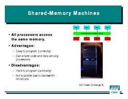 Shared memory machines allow all processors to access a global memory (or
several global memory modules). Information can be passed through this
memory, making programming easier.
However, making this global memory fast usually requires local cacheing of
data on the processors, so it is still a good idea to take advantage of
data locality.
Early languages for parallel machines reflected the underlying hardware
fairly strongly. Distributed memory machines typically forced the
programmer to identify both the sender and receiver of all messages, while
shared memory languages used barriers and signals to coordinate processors.
While this led to efficient programs, it also made programs non-portable.
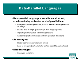 HPF uses data parallelism to allow users to write
portable parallel programs. The main idea is that the parallelism comes
from independent operations on all (or most) of the elements of large data
structures. Since HPF is based on Fortran 90, the data structures are
usually arrays. The parallel operations are often array arithmetic,
although we'll see later that this can be generalized somewhat. Since
there are typically tens (perhaps hundreds) of processors and thousands (or
millions) of array elements, the elements have to be divided among the
processors. HPF does this by high-level data mapping directives. The
HPF compiler uses these hints from the user to decide which processor
should perform each elemental operation. Basically, the compiler
schedules the computation so that as many elements are local to the
processor executing it as possible.
The next three sections of the tutorial look at the major pieces of HPF:
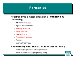
ALLOCATE statement
can allocate memory (including arrays) from the heap. This allows the
kind of structured memory management found in other modern languages. It
helps HPF by making it easier to declare arrays to be their "natural"
size (which in turn affects their mapping).SUM
and MAXVAL perform reductions on whole arrays. Other
intrinsics perform data movement (CSHIFT for circular shift)
and other useful operations (MATMUL for matrix multiplication).POINTER variables (more powerful than Pascal's pointers, but
more structured than C pointers), and record structures (called "derived
types").
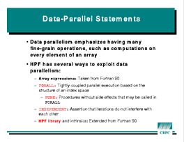
FORALL statement, a generalization of element-wise
array assignmentsPURE functions, which can be used within a FORALL
to provide larger-grain operationsINDEPENDENT directive, which asserts that a loop can
be executed in parallel.
 The
The FORALL statement was adapted from proposals made during
the Fortran 90 development process and from a popular feature of the
Connection Machine Fortran compiler.
While its form resembles a DO statement, its meaning is very
different.
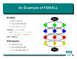
The FORALL statement
FORALL ( I = 2 : 4 )
    A(I) = A(I-1) + A(I+1)
    C(I) = B(I) * A(I+1)
END FORALL
executes as follows:
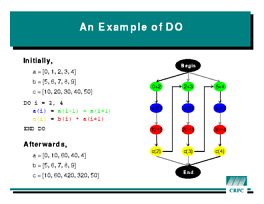
A(I-1) + A(I+1) for I = 2, 3,
and 4. (These are the green ovals in the picture at left.)A(I) locations.
(Blue ovals.)B(I) * A(I+1) for the three values of I.
(Red ovals)C(I) locations.
(Yellow ovals.)FORALL. Notice that, because there are no arrows across a
row, that all operations in one row can be performed in parallel. For
example, the three red ovals could each execute on a separate processor.
Because of the arrows between levels, however, there may have to
be synchronizations between the computations and the actual assignments.
 The
The FORALL example is different from the similar-looking
DO I = 1, 3
    A(I) = A(I-1) + A(I+1)
    C(I) = B(I) * A(I+1)
END DO
whose dependence diagram is shown at right.
Although there are fewer constraints in the DO loop, the ones
that are there are killers. Because of the arrow from the bottom
of each iteration to the top of the next, everything must be done exactly
in order. That is, nothing can run in parallel.
One other aspect of FORALL is hard to see in the small
figures. Many of the worst-case dependences in the FORALL do
not occur in any particular program; these are marked in gray, rather than black. If a
compiler can detect this, it can produce more efficient parallel
code by avoiding the synchronization points.
(The same is true of a DO loop; that's how
vectorizing compilers work.)
If you are familiar with Fortran 90, you may notice that FORALL
has the same semantics as an array assignment (or a series of array
assignments). In fact, any array assignment can be
written as a FORALL; however, FORALL can express
some array subsections, like diagonals, that array assignments can't.
In practice, FORALL is a convienient way to express many
array update operations.
Some users find it easier to understand than array assignments,
especially assignments to array subsections; others feel exactly the
opposite.
 One of the constraints on
 FORALL statements is that they can
only contain assignments. Conditionals, nested loops, and CALLs
are not
allowed. Also, it would be unsafe for a statement in a FORALL
to invoke an arbitrary function - if the function had side effects, the
results could be completely messed up.
These are both serious limitations on FORALL functionality,
and would probably be unacceptable to programmers.
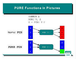
Therefore, HPF also introduces a new class of functions called
PURE functions which cannot have side effects.
The code inside the PURE function can have arbitrarily complex
control flow,
including conditionals and loops. However, it cannot assign to any global
variables or dummy arguments, nor can it use globals or dummies anywhere
that their values might change (for example, as a DO loop
index).
 The
The INDEPENDENT directive takes a different approach to
specifying data parallelism. Rather than define a new statement with new
semantics, INDEPENDENT gives the compiler more information
about existing Fortran statements. In particular, !HPF$ INDEPENDENT
before a DO loop tells the compiler that the iterations of
the loop do not affect each other in any way. (The !HPF$
means that INDEPENDENT is advice to the compiler, rather than a
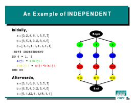
first-class statement.) So the code block
!HPF$ INDEPENDENT
DO J = 1, 3
    A(J) = A( B(J) )
    C(J) = A(J) * B(A(J))
END DO
can be run with each iteration on a separate processor and no
synchronization during the loop. The worst-case dependence diagram for
this loop is
shown at right. Again, it is possible for some of the dependence arcs to
be missing in a particular case, but it is less common for compilers to
try to take advantage of this.
Instead, HPF compilers concentrate on partitioning the iterations between
processors. A common heuristic for this is the "owner-computes rule," in
which the processor that owns one of the left-hand sides takes
responsibility for all computations in an iteration.
INDEPENDENT is most useful for giving the compiler
application-specific knowledge that can be used to run a loop in parallel.
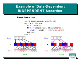
For example, the figure at left illustrates the code segment
!HPF$ INDEPENDENT, NEW(J)
DO I = 1, N
  DO J = IBEGIN(I), IEND(I)
    X(IBLUE(I)) = X(IBLUE(I)) + X(IRED(J))
  END DO
END DO
(The NEW clause means that J is local to the
outer loop.)
The programmer is telling the compiler that the elements X(IBLUE(I))
and X(IRED(J)) are distinct for all values of I
and J. Also, the IBLUE array cannot have any
repeated values. Essentially, IBLUE and IRED
arrays
have to partition the X array as shown in the lower left.
This is enough for the compiler to run the outer loop in parallel. It is
also information that the compiler could not discover on its
own; it depends on the input data (and, presumably, on the program's data
structures and algorithms).
If
IBLUE and IRED don't correctly partition the
array (shown on the lower right), then it is a programming error.
Unfortunately, it will be a difficult error to find.
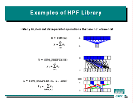 The HPF library and intrinsics are the final set of data-parallel features
in the language. These are operations that have 3 important properties:
SUM at the top of the
figure; actually a Fortran 90 intrinsic), prefix operators
(SUM_PREFIX in the middle; each element is the sum of the
elements before it), and scatter operators (SUM_SCATTER at
the bottom; arbitrary shuffling and combining of data). In addition, HPF
offers sorting functions in the library.
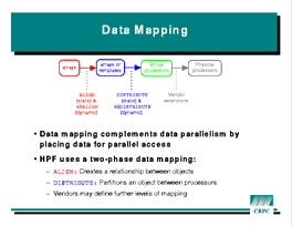
ALIGN directive does fine-grain matching between separate
arrays; when two array elements are aligned together, they will always be
stored on the same processorDISTRIBUTE directive partitions an array among
processors; this mapping "drags along" any other arrays aligned with it.ALIGN
and use DISTRIBUTE for all their arrays.
 The
The DISTRIBUTE directive partitions an array by specifying a
regular distribution pattern for each dimension.
The basic form of a DISTRIBUTE directive on a 2-dimensional
array is
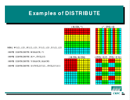
!HPF$ DISTRIBUTE array_name(pattern1, pattern2)The figure at left shows four possible distributions of a 12 by 12 array by giving elements on the same processor the same color. The
BLOCK
pattern breaks the dimension into equal-sized blocks, one per processor.
For example, the
upper left array in the figure uses a BLOCK distribution on rows. The
CYCLIC pattern is at the other end of the spectrum - it
spreads the elements one per processor, wrapping around
when it runs out of processors. The upper left array is CYCLIC
in the column dimension.
Dimensions that are not divided between processors are denoted by
*. Therefore, the declarations for the top two arrays are
!HPF$ DISTRIBUTE A(BLOCK,*)
!HPF$ DISTRIBUTE B(*,CYCLIC)
CYCLIC can also take a parameter K,
which causes it to dole out
groups of K instead of single elements.
The lower right array therefore uses the pattern
(CYCLIC(2),CYCLIC(3). The (extremely common) distribution at
lower left is (BLOCK,BLOCK).
The purpose of choosing a distribution is to control the performance of the
code. Because of the owner-computes strategy of most HPF
compilers, the dimension(s) of an array with the most potential data
parallelism should be divided among processors (i.e. they should use a
pattern other than *). This will assure that operations that
can run in parallel will run in parallel.
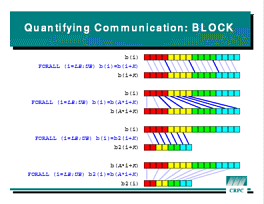 To decide which pattern to use, you need to consider the data movement that
will be generated. The goal is to minimize the amount of data that has to
move between processors. (Even on shared memory machines, data may have
to move from one processor's cache to another's cache.) The figure at
right shows how to estimate this graphically. Consider which elements are
used together (for example, appear in the same expression). If the
elements are on the same processor, there should not be data movement; if
they are on different processors, at least one of them must move. The
figure uses color-coding for processors, and shows communications
as dark lines for several common subscript patterns. Although the
analysis can become tedious, the following rules of thumb cover many
programs:
BLOCK distribution is good for nearest-neighbor
communication, such as local stencils on regular meshes.N and c*N (where
c is a compile-time constant), BLOCK (for both
arrays) works well for linear interpolation (e.g. A(I) =
B(I*c)) between the arrays.CYCLIC (or CYCLIC(k)) is good for load
balancing, but does not preserve data locality between nearest neighbors.CYCLIC creates data locality for long-stride accesses
(e.g. A(I) * A(I+64)) if the stride is a multiple
of the number of processors. (This occurs in practice in recursive
doubling algorithms on machines with a power of 2 processors.)
The ALIGN directive matches individual array elements to other
array elements or to slices of arrays.
The syntax is
!HPF$ ALIGN array1(i,j) with array2(i*a+b, j*c-d)Given this directive, only
array2 can appear in a
DISTRIBUTE directive.
The "dummy arguments" on aray1 can be any integer variables,
and the expressions after array2 can be any affine linear functions
of the dummies. In many programs, the linear functions are simply the
dummy arguments; that is, ALIGN uses an identity mapping
rather than a more complex one. ALIGN can also use the
* to represent "all values in that dimension". This allows
replication of array elements across several processors.
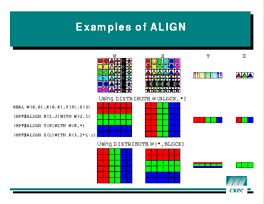
!HPF$ ALIGN X(I,J) WITH W(J,I)
!HPF$ ALIGN Y(K) WITH W(K,*)
!HPF$ ALIGN Z(L) WITH X(3,2*L-1)
Elements are mapped together if they contain the same symbol in the same color. (This is much easier to see in the full-size slide.) So,
X is aligned with the transpose of W;
X(1,6) and W(6,1) both contain a magenta square.
Each element of Y is aligned with an entire row of
W, so Y(2) contains six yellow symbols
corresponding to the six yellow elements in W's second row.
Z is ultimately aligned to every other element in
W's third column, that is to three of the six colored
triangles. The lower two-thirds of the figure shows the effect on all
arrays of two distributions for W.
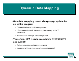 Two extensions of the above distribution mechanism are important to HPF.
The first is dynamic data mapping. For some arrays, a single distribution
is not appropriate for the entire program. For example, an efficient
2-dimensional FFT might distribute the array by rows to process the X
dimension, then distribute the array by columns to perform the Y-direction
operations. Another example is using runtime information (such as the
size of an array) to pick the appropriate mapping.
Recognizing this need, HPF provides "executable" versions of the
ALIGN and DISTRIBUTE directives called
REALIGN and REDISTRIBUTE. The syntax and
semantics are the same as for the "declaration" directives, except that
the new forms apply from the time it is executed until another mapping
directive is encountered. That is, the "RE" forms have
dynamic scope while the normal forms have static scope. Users should be
aware, however, that REALIGN and REDISTRIBUTE
will generally cause heavy data movement if they are used.
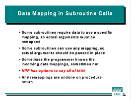 The other extension to the basic mapping capabilities applies to dummy
arguments. There are several things that one might want to do with a
dummy's mapping:
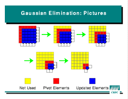 Gaussian elimination illustrates array
operations and load balancing for dense linear algebra. The algorithm
solves a system of linear equations by successively updating the matrix
that represents the system. The figure at left shows the pattern of these
updates: at each stage, the blue section of the array is
updated using its own values and the values of the red elements. The
updating operation itself is data-parallel, and thus a good choice for
HPF. There is no data locality in the computation, since each red element
updates several blue ones. However, since the amount of work shrinks at
each stage, it is important to choose a distribution that keeps as many
processors busy as possible. In this case, that is the
 CYCLIC
data distribution.
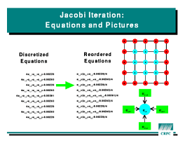 Jacobi iteration illustrates nearest-neighbor communication. The algorithm
solves a simple PDE by discretizing it on a regular mesh and approximating
the equation at each mesh point by a finite difference form. The resulting
set of equations are solved iteratively by updating each array element
using the stencil shown in the figure. Again, this is a classically
data-parallel operation. Unlike Gaussian elimination, however, there is
substantial data locality and no load imbalance to worry about. Such
computations' performance is optimized by HPF's
 BLOCK
distribution.
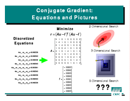 Conjugate gradient expands
Jacobi to a more realistic numerical method.
The new method uses the same discretization and finite difference
formulation as before, but formulates the problem as an error minimization.
This allows some sophisticated mathematics to be brought to bear on the
problem, leading to a much more efficient iterative scheme. Each
iteration of the conjugate gradient iteration requires a Jacobi-like
computation of the residual, two dot products, and several vector updates.
All these operations are data-parallel. The best data distribution is
determined by the residual, prompting the use of
 BLOCK
distribution here. More complex problems could be solved by the conjugate
gradient method by replacing the residual routine and choosing a data
distribution appropriate to the new operator.
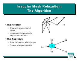 Finally, relaxation on an irregular mesh
shows what is (and what is not) supported in HPF for irregular
computations. The algorithm updates the nodes in a graph based on values
stored in the edges. The data parallelism is trickier here than in the
previous examples, since each node may be updated by several edges.
However, the HPF library routine
 SUM_SCATTER performs this
operation efficiently. The cost of the scatter will depend on how the
nodes and edges are mapped to processors. Conceptually, one would like
to place the nodes individually. However, this is not possible with HPF's
regular distributions. What is possible is to renumber the nodes so that
nodes near each other in the graph are also near each other in the array.
After this permutation, a simple BLOCK distribution will tend
to enhance data locality.
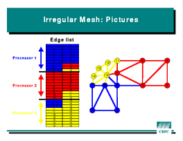 Similarly, the edges can be reordered so they
land on the same processor as their endpoints. Such a reordered mesh is
shown in the figure at left. While this example shows that irregular
computations are possible in HPF, it is clear the the program is far from
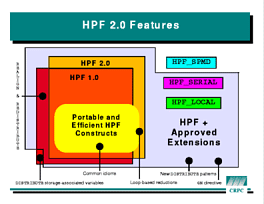
elegant. Some of the extensions under development for HPF 2 address these
issues.

Back to
main tutorial
Chuck Koelbel